
One can estimate the value of Pi using Monte Carlo technique. The procedure is really intuitive and based on probabilities and random number generation. I have already written a lot about random number generation in my old posts.
So here’s what we do.
We consider a square extending from x=-1 to x=1 and y=-1 to y=1. That is each side is 2 units long. Now we inscribe a circle of radius 1 unit inside this square, such that the centre of the circle and the square both are at origin. Now, let’s say you drop pins/needles/rice grains or any other thing on the square randomly.
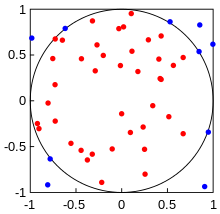
The process of dropping the pins should be completely random and all positions for the landing of the pin should be equally probable. If this is the case, then we can say that the number of pins falling inside the circle (Nc) divided by the total no. of pins dropped on the square (Nt) is given by:
That is the probability of the pin falling inside the circle is directly proportional to the area of the circle. I hope this step is intuitive enough for you.
Well, that’s it. The above relation basically gives you the value of Pi. How?
Well, the area of circle in our case is just 
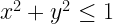
So if we write a program that randomly generates x and y coordinates of the falling pin such that 

Then the coordinates of the pins that fall inside the circle would satisfy the following relation.
Thus we can count the number of pins falling inside the circle, by incrementing a counter whenever the above relation is satisfied. Finally we can take the ratios of the pins falling inside the circle to the total no. of pins that were made to fall, and use the equation mentioned above to get the value of pi.
The following program illustrates the procedure:
Python Code:
# Author: Manas Sharma
# Website: www.bragitoff.com
# Email: [email protected]
# License: MIT
# Value of Pi using Monte carlo

import numpy as np


# Input parameters
nTrials = int(10E4)
radius = 1
#-------------
# Counter for thepoints inside the circle
nInside = 0

# Generate points in a square of side 2 units, from -1 to 1.
XrandCoords = np.random.default_rng().uniform(-1, 1, (nTrials,))
YrandCoords = np.random.default_rng().uniform(-1, 1, (nTrials,))

for i in range(nTrials):
    x = XrandCoords[i]
    y = YrandCoords[i]
    # Check if the points are inside the circle or not
    if x**2+y**2<=radius**2:
        nInside = nInside + 1


area = 4*nInside/nTrials
print("Value of Pi: ",area)
OUTPUT:
Value of Pi: 3.14152
Now, that we have seen that the above code works, we can also try to make a pretty animated simulation demonstrating the process.
Monte Carlo animation Python Code:
# Author: Manas Sharma
# Website: www.bragitoff.com
# Email: [email protected]
# License: MIT
# Value of Pi using Matplotlib animation

import numpy as np
import matplotlib
matplotlib.use("TkAgg") # set the backend (to move the windows to desired location on screen)
import matplotlib.pyplot as plt
# from matplotlib.pyplot import figure
from matplotlib.pyplot import *

fig = figure(figsize=(8, 8), dpi=120)


# Input parameters
nTrials = int(1E4)
radius = 1
#-------------
# Counter for the pins inside the circle
nInside = 0
# Counter for the pins dropped
nDrops = 0

# Generate points in a square of side 2 units, from -1 to 1.
XrandCoords = np.random.default_rng().uniform(-1, 1, (nTrials,))
YrandCoords = np.random.default_rng().uniform(-1, 1, (nTrials,))

# First matplotlib window
fig1 = plt.figure(1)
plt.get_current_fig_manager().window.wm_geometry("+00+00") # move the window
plt.xlim(-1,1)
plt.ylim(-1,1)
plt.legend()

# Second matplotlib window
plt.figure(2)
plt.get_current_fig_manager().window.wm_geometry("+960+00") # move the window
# plt.ylim(2.8,4.3)

# Some checks so the legend labels are only drawn once
isFirst1 = True
isFirst2 = True

# Some arrays to store the pi value vs the number of pins dropped
piValueI = []
nDrops_arr = []

# Some arrays to plot the points
insideX = []
outsideX = []
insideY = []
outsideY = []

# Begin Monte Carlo
for i in range(nTrials):
    x = XrandCoords[i]
    y = YrandCoords[i]
    # Increment the counter for number of total pins dropped
    nDrops = nDrops + 1


    # Check if the points are inside the circle or not
    if x**2+y**2<=radius**2:
        nInside = nInside + 1
        insideX.append(x)
        insideY.append(y)

    else:
        outsideX.append(x)
        outsideY.append(y)


    # plot only at some values
    if i%100==0:
        # Draw on first window
        plt.figure(1)
        # The label is only needed once so
        if isFirst1:

            # Plot once with label
            plt.scatter(insideX,insideY,c='pink',s=50,label='Drop inside')
            isFirst1 = False
            plt.legend(loc=(0.75, 0.9))
        else:
            #Remaining plot without label
           plt.scatter(insideX,insideY,c='pink',s=50)
        # Draw on first window
        plt.figure(1)
        # The label is only needed once so
        if isFirst2:
            # Plot once with label
            plt.scatter(outsideX,outsideY,c='orange',s=50,label='Drop outside')
            isFirst2 = False
            plt.legend(loc=(0.75, 0.9))
        else:
            #Remaining plot without label
           plt.scatter(outsideX,outsideY,c='orange',s=50)


        area = 4*nInside/nDrops
        plt.figure(1)
        plt.title('No. of pin drops = '+str(nDrops)+';         No. inside circle = '+str(nInside)+r';         π  ≈ $4\frac{N_\mathrm{inside}}{N_\mathrm{total}}=$ '+str(np.round(area,6)))
        piValueI.append(area)
        nDrops_arr.append(nDrops)
        # For plotting on the second window
        plt.figure(2)
        plt.axhline(y=np.pi, c='darkseagreen',linewidth=2,alpha=0.5)
        plt.plot(nDrops_arr,piValueI,c='mediumorchid')
        plt.title('π estimate vs no. of pin drops')
        plt.annotate('π',[0,np.pi],fontsize=20)
        # The following command is needed to make the second window plot work.
        plt.draw()
        # Pause for animation
        plt.pause(0.1)


area = 4*nInside/nTrials
print("Final estimated value of Pi: ",area)


plt.show()
OUTPUT:
References:
https://en.wikipedia.org/wiki/Monte_Carlo_method
I’m a physicist specializing in computational material science with a PhD in Physics from Friedrich-Schiller University Jena, Germany. I write efficient codes for simulating light-matter interactions at atomic scales. I like to develop Physics, DFT, and Machine Learning related apps and software from time to time. Can code in most of the popular languages. I like to share my knowledge in Physics and applications using this Blog and a YouTube channel.