Electronic correlation refers to the interactions between electrons within the electronic structure of a quantum system. In fact, the correlation energy from a correlated quantum chemistry method can tell how much the motion of one electron is coupled to the motion of all other electrons in a quantum system. In this blog post, we will explore the concept of electron correlation, its significance, and how it impacts quantum chemistry methods like Hartree Fock.

To comprehend electron correlation, let’s consider an example.

If the electrons were truly independent, the probability of finding electron 1 in position A would be completely unrelated to whether electron 2 is in position X or not – similar to flipping two coins where the outcome of one flip does not influence the other.

However, electrons have negative charges and therefore repel each other. If electron 1 occupies orbital A, it becomes much less likely to find electron 2 in orbital X which spatially overlaps with A. In this way, the electrons’ motions and locations are correlated. We can also think of this analogy in terms of people occupying adjacent seats in a theater – if person 1 sits in seat A, it affects the probability that person 2 will sit in the neighboring seat B. The presence of person 1 affects the position of person 2.

This electronic correlation poses a major challenge for solving the electronic Schrödinger equation (for an -electron system):

where is the wavefunction containing all the system’s quantum mechanical information and is a function of the electrons’ spatial coordinates (spin is neglected here for simplicity), is the energy, and is the Hamiltonian operator representing the total energy.

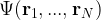
The Hamiltonian for a multi-electron system is given as

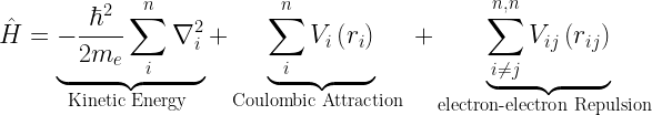
The first term in the Hamiltonian corresponds to the kinetic energy and the second term to the nuclear-electron interaction (attractive).

It is the third term, in the above equation, that makes life problematic. It accounts for the electron-electron repulsion that is expected for same charged particles and is responsible for electron correlation. It makes it impossible to solve the Schrödinger equation exactly for systems with 2 or more electrons. Yes! you read it right. Even the Schrödinger equation for Helium atom cannot be solved analytically without using some approximations. This is because the Hamiltonian of Helium atom represents a three-body problem – in fact a  quantum three-body problem, which is not going to be easier than a classical one. The problem with such multi-electron systems is that there aren’t any tricks that we can employ to separate it into simpler constituents which we can solve individually, as in the case of Hydrogen atom.

The Coulomb repulsion term is also the reason why the wavefunction of the N-electron system depends on the spatial coordinates of all the N electrons simultaneously (Note: Spin has not been considered here for simplicity).

In three dimensions, the exact wavefunction is a function of variables as each electron has 3 degrees of freedom. This makes the exact wavefunction an intractable high-dimensional object even when employing numerical techniques and using supercomputers. For example, if you were to try to store the wavefunction, using a very modest discretization of 10 grid points along each spatial dimension, a simple medium-sized Iron (Fe) atom (26-electron system) would require or numerical values per wavefunction – already demanding an unfathomable amount of storage (more than the entire content of the internet).

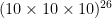
To avoid this “curse of dimensionality”, quantum chemists resort to approximations. One such approximation is the Hartree approximation which assumes that the total wavefunction can be written as a simple product of single-electron wavefunctions (also referred to as a Hartree product):

.

This greatly alleviates computational costs, since the problem reduces to solving independent Schrödinger equations, each with only 3 spatial variables. However, writing the wavefunction as a Hartree product means that the probability density for each electron becomes completely independent. For a 2-electron system, the probability of finding electron 1 at no longer depends on the position of electron 2. In other words,

Consequently, this Hartree product loses electron correlation effects.

One thing that has been completely ignored in the Hartree approximation is that electrons are indistinguishable quantum particles. Therefore, the wavefunction should be antisymmetric (change sign) with respect to the interchange of two electrons. The Hartree approximation is therefore improved upon by the Hartree-Fock (HF) method, where the -body wavefunction ( denotes both spatial and spin coordinates {}) is approximated by a single Slater determinant rather than a simple product.

In the above equation, are the spin orbitals and are the spatial and spin coordinates.

This results in a fermionic exchange term in the Hamiltonian operator which enforces the Pauli exclusion principle, i.e., prevents two electrons with the same spin from being found in the same location. Hence, the HF method partially accounts for electron correlation, specifically Fermi correlation, due to the spin of electrons. Coulomb correlation, on the other hand, describes the correlation between the spatial positions of electrons due to their Coulomb repulsion and the HF method fails to capture it, as it considers the interaction of every electron with the mean field of all other electrons, rather than considering the instantaneous repulsion between electrons. The Coulomb correlation is responsible for chemically important effects such as London dispersion.

Therefore, usually the correlation energy is also defined as the difference between the exact energy (obtained by solving the Schrödinger equation exactly) and the HF energy.  (Although note that some portion of the correlation energy due to spin is included in HF)

.

In quantum chemistry, various post-Hartree-Fock methods have been developed to account for electron correlation. Some examples include Configuration Interaction, Møller–Plesset perturbation theory (MP2, MP3, MP4, etc.), and coupled cluster methods. These methods are typically implemented for molecular systems and can now be extended to small periodic systems using tools like PySCF. In the context of correlated quantum chemistry methods, the correlation energy is defined as the energy difference relative to HF energy. But this is highly dependent on the basis set used.

Density functional theory (DFT) is another widely used approach in quantum chemistry. It accounts for electron correlation through the exchange-correlation functional, which approximates the exchange and correlation effects. Additionally, the DFT+ method can be employed to incorporate electron correlation effects. DFT+ introduces an on-site Coulomb repulsion term (known as ) to more accurately account for strong on-site electron-electron repulsion. This term is applied to the localized electron states usually associated with the or orbitals. By tuning the parameter, DFT+ can obtain improved agreement with experiments compared to standard DFT methods when looking at properties that depend strongly on electron correlations. This includes properties like band gaps, magnetic moments, charge ordering, metal-insulator transitions etc.

It is also worth noting that correlation can also be categorized as static or dynamic correlation.

Dynamic correlation arises from the fact that electrons in the HF model do not interact instantaneously with each other, unlike in reality. In the HF model, each electron interacts with the average field created by all other electrons, and the model fails to accurately capture the instantaneous interactions between electrons. This deficiency in reproducing the dynamic motion of electrons contributes to dynamic correlation effects. Methods like Møller-Plesset perturbation theory (MPn) are examples that primarily address dynamic correlation.

On the other hand, static correlation is related to the use of only a single Slater determinant as an approximation to the wavefunction in the HF model. In certain cases an electronic state can be well described only by a linear combination of more than one (nearly-)degenerate Slater determinants.  In such cases where multiple determinants are needed, static correlation effects become prominent. The multi-configurational self-consistent field (MCSCF) method is an example of a technique that primarily accounts for static correlation.

Take note of the term “primarily” mentioned above. In principle, it’s difficult to exactly isolate dynamic and static correlation effects because both emerge from the same physical interactions. Consequently, approaches designed to account for dynamic correlation effects often end up incorporating aspects of non-dynamic correlation effects at higher orders, and the reverse is also true.

References

1. Electronic correlation – Wikipedia
2. Amazon.com: Modern quantum chemistry: Introduction to advanced electronic structure theory: 9780029497104: Szabó, Attila: Books
3. theoretical chemistry – What is the difference between dynamic and static electronic correlation – Chemistry Stack Exchange
4. How does static correlation differ from Fermi correlation, and how does dynamic correlation differ from Coulomb correlation? – Matter Modeling Stack Exchange
5. Intro to DFT – Day 1: Density-functional theory – Nicola Marzari – YouTube
6. 6.7: The Helium Atom Cannot Be Solved Exactly – Chemistry LibreTexts
7. quantum mechanics – Does a solution for Helium atom not exist or is it too difficult to find analytically? – Physics Stack Exchange
8. quantum mechanics – Why are analytical solutions of the Schrödinger equation available only for a small number of simple models? – Physics Stack Exchange
9. intro-e-correlation.dvi (gatech.edu)