
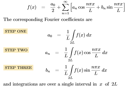
Today I wrote a code that calculates the Fourier Coefficients.
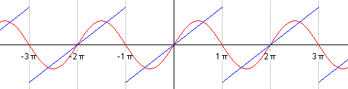
In case you don’t know what a Fourier Series is, then, basically it is a way of approximating or representing a periodic function by a series of simple harmonic(sine and cosine) functions.
You can check out the wikipedia for more information on it: https://en.wikipedia.org/wiki/Fourier_series
So, here’s how my code works:
I created a function ‘Fourier’ that takes in 4 arguments.
First two arguments specify the range for which the original function that is to be approximated is defined for. These are indicated as li (initial limit),lf (final limit).
The third argument ‘n’ is the number of harmonic terms to be used. (Larger the ‘n’ => better the approximation.)
And the final argument is the function ‘f’ which is to be approximated.
The function returns the Fourier coefficients based on formula shown in the above image. The coefficients are returned as a python list: [a0/2,An,Bn].
a0/2 is the first Fourier coefficient and is a scalar.
An and Bn are numpy 1d arrays of size n, which store the coefficients of cosine and sine terms respectively.
To calculate these coefficients I perform integration using the script.integrate module.
CODE
#Fourier Series Coefficients
#The following function returns the fourier coefficients,'a0/2', 'An' & 'Bn'
#
#User needs to provide the following arguments:
#
#l=periodicity of the function f which is to be approximated by Fourier Series
#n=no. of Fourier Coefficients you want to calculate
#f=function which is to be approximated by Fourier Series
#
#*Some necessary guidelines for defining f:
#*The program integrates the function f from -l to l so make sure you define the function f correctly in the interval -l to l.
#
#for more information on Fourier Series visit: https://en.wikipedia.org/wiki/Fourier_series
#
#Written by: Manas Sharma([email protected])
#For more useful toolboxes and tutorials on Python visit: https://www.bragitoff.com/category/compu-geek/python/
def fourier(li, lf, n, f):
    l = (lf-li)/2
    # Constant term
    a0=1/l*integrate.quad(lambda x: f(x), li, lf)[0]
    # Cosine coefficents
    A = np.zeros((n))
    # Sine coefficents
    B = np.zeros((n))

    for i in range(1,n+1):
        A[i-1]=1/l*integrate.quad(lambda x: f(x)*np.cos(i*np.pi*x/l), li, lf)[0]
        B[i-1]=1/l* integrate.quad(lambda x: f(x)*np.sin(i*np.pi*x/l), li, lf)[0]

    return [a0/2.0, A, B]
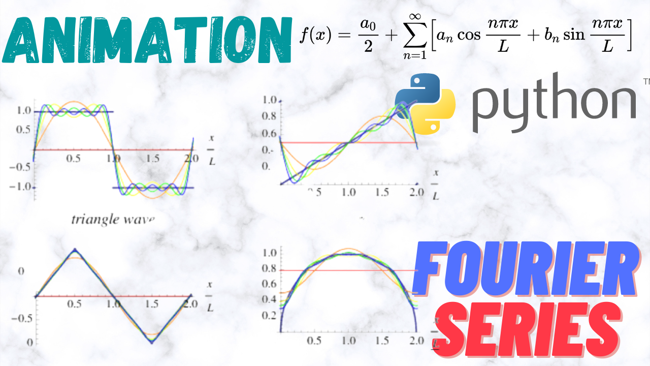
Now, let’s have a look at some real world examples. The following program can be used to approximate 4 popular periodic functions using the Fourier series. Just copy and paste it to run and play with it yourself.
# Author: Manas Sharma
# Website: www.bragitoff.com
# Email: [email protected]
# License: MIT

import numpy as np
import scipy.integrate as integrate


# Non-periodic sawtooth function defined for a range [-l,l]
def sawtooth(x):
    return x


# Non-periodic square wave function defined for a range [-l,l]
def square(x):
    if x>0:
        return np.pi
    else:
        return -np.pi


# Non-periodic triangle wave function defined for a range [-l,l]
def triangle(x):
    if x>0:
        return x
    else:
        return -x


# Non-periodic cycloid wave function defined for a range [-l,l]
def cycloid(x):
    return np.sqrt(np.pi**2-x**2)

#Fourier Series Coefficients
#The following function returns the fourier coefficients,'a0/2', 'An' & 'Bn'
#
#User needs to provide the following arguments:
#
#l=periodicity of the function f which is to be approximated by Fourier Series
#n=no. of Fourier Coefficients you want to calculate
#f=function which is to be approximated by Fourier Series
#
#*Some necessary guidelines for defining f:
#*The program integrates the function f from -l to l so make sure you define the function f correctly in the interval -l to l.
#
#for more information on Fourier Series visit: https://en.wikipedia.org/wiki/Fourier_series
#
#Written by: Manas Sharma([email protected])
#For more useful tutorials on Python visit: https://www.bragitoff.com/category/compu-geek/python/
def fourier(li, lf, n, f):
    l = (lf-li)/2
    # Constant term
    a0=1/l*integrate.quad(lambda x: f(x), li, lf)[0]
    # Cosine coefficents
    A = np.zeros((n))
    # Sine coefficents
    B = np.zeros((n))

    for i in range(1,n+1):
        A[i-1]=1/l*integrate.quad(lambda x: f(x)*np.cos(i*np.pi*x/l), li, lf)[0]
        B[i-1]=1/l* integrate.quad(lambda x: f(x)*np.sin(i*np.pi*x/l), li, lf)[0]

    return [a0/2.0, A, B]

if __name__ == "__main__":


    # Limits for the functions
    li = -np.pi
    lf = np.pi

    # Number of harmonic terms
    n = 3

    # Fourier coeffficients for various functions
    coeffs = fourier(li,lf,n,sawtooth)
    print('Fourier coefficients for the Sawtooth wave\n')
    print('a0 ='+str(coeffs[0]))
    print('an ='+str(coeffs[1]))
    print('bn ='+str(coeffs[2]))
    print('-----------------------\n\n')

    coeffs = fourier(li,lf,n,square)
    print('Fourier coefficients for the Square wave\n')
    print('a0 ='+str(coeffs[0]))
    print('an ='+str(coeffs[1]))
    print('bn ='+str(coeffs[2]))
    print('-----------------------\n\n')

    coeffs = fourier(li,lf,n,triangle)
    print('Fourier coefficients for the Triangular wave\n')
    print('a0 ='+str(coeffs[0]))
    print('an ='+str(coeffs[1]))
    print('bn ='+str(coeffs[2]))
    print('-----------------------\n\n')

    coeffs = fourier(li,lf,n,cycloid)
    print('Fourier coefficients for the Cycloid wave\n')
    print('a0 ='+str(coeffs[0]))
    print('an ='+str(coeffs[1]))
    print('bn ='+str(coeffs[2]))
    print('-----------------------\n\n')
OUTPUT:
>>   python3 fourier.py
Fourier coefficients for the Sawtooth wave

a0 =0.0
an =[0. 0. 0.]
bn =[ 2.         -1.          0.66666667]
-----------------------


Fourier coefficients for the Square wave

a0 =0.0
an =[0. 0. 0.]
bn =[4.00000000e+00 3.11674695e-16 1.33333333e+00]
-----------------------


Fourier coefficients for the Triangular wave

a0 =1.5707963267948966
an =[-1.27323954e+00  4.99600361e-16 -1.41471061e-01]
bn =[0. 0. 0.]
-----------------------


Fourier coefficients for the Cycloid wave

a0 =2.4674011002723417
an =[ 0.89414547 -0.3336097   0.1850662 ]
bn =[0. 0. 0.]
-----------------------
It is quite evident, how the coefficients of sine terms are 0 if the function is even (triangular wave, cycloid), and the coefficients of cosine terms are 0 if the function is odd (square wave, sawtooth wave).
Now, let us try to visualise these results with the help of an animation created using the following Python code:
ANIMATION CODE:
# Author: Manas Sharma
# Website: www.bragitoff.com
# Email: [email protected]
# License: MIT

import numpy as np
import matplotlib.pyplot as plt
from matplotlib.pyplot import *
import scipy.integrate as integrate

fig = figure(figsize=(7, 7), dpi=120)


# Function that will convert any given function 'f' defined in a given range '[li,lf]' to a periodic function of period 'lf-li'
def periodicf(li,lf,f,x):
    if x>=li and x<=lf :
        return f(x)
    elif x>lf:
        x_new=x-(lf-li)
        return periodicf(li,lf,f,x_new)
    elif x<(li):
        x_new=x+(lf-li)
        return periodicf(li,lf,f,x_new)

# The periodic version of sawtooth function
def sawtoothP(li,lf,x):
    return periodicf(li,lf,sawtooth,x)

# Non-periodic sawtooth function defined for a range [-l,l]
def sawtooth(x):
    return x

# The periodic version of square function
def squareP(li,lf,x):
    return periodicf(li,lf,square,x)

# Non-periodic square wave function defined for a range [-l,l]
def square(x):
    if x>0:
        return np.pi
    else:
        return -np.pi

# The periodic version of triangle function
def triangleP(li,lf,x):
    return periodicf(li,lf,triangle,x)

# Non-periodic triangle wave function defined for a range [-l,l]
def triangle(x):
    if x>0:
        return x
    else:
        return -x

# The periodic version of cycloid function
def cycloidP(li,lf,x):
    return periodicf(li,lf,cycloid,x)

# Non-periodic cycloid wave function defined for a range [-l,l]
def cycloid(x):
    return np.sqrt(np.pi**2-x**2)

#Fourier Series Coefficients
#The following function returns the fourier coefficients,'a0/2', 'An' & 'Bn'
#
#User needs to provide the following arguments:
#
#li,lf = Range over which the original function f which is to be approximated by Fourier Series is defined. Period is assumed to be lf-li
#n=no. of Fourier Coefficients you want to calculate
#f=function which is to be approximated by Fourier Series
#
#*Some necessary guidelines for defining f:
#*The program integrates the function f from li to lf so make sure you define the function f correctly in the interval li to lf.
#
#for more information on Fourier Series visit: https://en.wikipedia.org/wiki/Fourier_series
#
#Written by: Manas Sharma([email protected])
#For more useful toolboxes and tutorials on Python visit: https://www.bragitoff.com/category/compu-geek/python/
def fourierCoeffs(li, lf, n, f):
    l = (lf-li)/2
    # Constant term
    a0=1/l*integrate.quad(lambda x: f(x), li, lf)[0]
    # Cosine coefficents
    A = np.zeros((n))
    # Sine coefficents
    B = np.zeros((n))

    for i in range(1,n+1):
        A[i-1]=1/l*integrate.quad(lambda x: f(x)*np.cos(i*np.pi*x/l), li, lf)[0]
        B[i-1]=1/l*integrate.quad(lambda x: f(x)*np.sin(i*np.pi*x/l), li, lf)[0]

    return [a0/2.0, A, B]

# This functions returns the value of the Fourier series for a given value of x given the already calculated Fourier coefficients
def fourierSeries(coeffs,x,l,n):
    value = coeffs[0]
    for i in range(1,n+1):
        value = value + coeffs[1][i-1]*np.cos(i*np.pi*x/l) +  coeffs[2][i-1]*np.sin(i*np.pi*x/l)
    return value


if __name__ == "__main__":

    # plt.style.use('dark_background')
    plt.style.use('seaborn')


    # Limits for the functions
    li = -np.pi
    lf = np.pi
    l = (lf-li)/2.0

    # Number of harmonic terms
    n = 1
    for n in range(1,10):

        plt.title('Fourier Series Approximation\nSawtooth Wave\n n = '+str(n))
        # plt.title('Fourier Series Approximation\nSquare Wave\n n = '+str(n))
        # plt.title('Fourier Series Approximation\nTriangular Wave\n n = '+str(n))
        # plt.title('Fourier Series Approximation\nCycloid\n n = '+str(n))

        # Fourier coeffficients for various functions
        coeffsSawtooth = fourierCoeffs(li,lf,n,sawtooth)
        coeffsTriangle = fourierCoeffs(li,lf,n,triangle)
        coeffsSquare = fourierCoeffs(li,lf,n,square)
        coeffsCycloid = fourierCoeffs(li,lf,n,cycloid)


        # Step size for plotting
        step_size = 0.05

        # Limits for plotting
        x_l = -np.pi*2
        x_u = np.pi*2

        # Sample values of x for plotting
        x = np.arange(x_l,x_u,step_size)
        y1 = [sawtoothP(li,lf,xi) for xi in x]
        y1_fourier = [fourierSeries(coeffsSawtooth,xi,l,n) for xi in x]
        y2 = [squareP(li,lf,xi) for xi in x]
        y2_fourier = [fourierSeries(coeffsSquare,xi,l,n) for xi in x]
        y3 = [triangleP(li,lf,xi) for xi in x]
        y3_fourier = [fourierSeries(coeffsTriangle,xi,l,n) for xi in x]
        y4 = [cycloidP(li,lf,xi) for xi in x]
        y4_fourier = [fourierSeries(coeffsCycloid,xi,l,n) for xi in x]

        x_plot =[]
        # Sawtooth
        y_plot1 = []
        y_plot1_fourier = []
        # Square
        y_plot2 = []
        y_plot2_fourier = []
        # Triangle
        y_plot3 = []
        y_plot3_fourier = []
        # Cycloid
        y_plot4 = []
        y_plot4_fourier = []

        x_l_plot = x_l - 13
        x_u_plot = x_l_plot + 14
        plt.xlim(x_l_plot,x_u_plot)
        plt.ylim(-6,7)

        for i in range(x.size):

            x_plot.append(x[i])
            # Actual function values
            y_plot1.append(y1[i])
            y_plot2.append(y2[i])
            y_plot3.append(y3[i])
            y_plot4.append(y4[i])
            # Values from fourier series
            y_plot1_fourier.append(y1_fourier[i])
            y_plot2_fourier.append(y2_fourier[i])
            y_plot3_fourier.append(y3_fourier[i])
            y_plot4_fourier.append(y4_fourier[i])

            #Sawtooth
            plt.plot(x_plot,y_plot1,c='darkkhaki',label='Sawtooth Wave')
            plt.plot(x_plot,y_plot1_fourier,c='forestgreen',label='Fourier Approximation')
            #Square
            #plt.plot(x_plot,y_plot2,c='tomato',label='Square Wave')
            #plt.plot(x_plot,y_plot2_fourier,c='maroon',label='Fourier Approximation')
            #Triangular
            #plt.plot(x_plot,y_plot3,c='orange',label = 'Triangular Wave')
            #plt.plot(x_plot,y_plot3_fourier,c='darkgoldenrod',label='Fourier Approximation')
            #Cycloid
            # plt.plot(x_plot,y_plot4,c='slateblue',label='Cycloid')
            # plt.plot(x_plot,y_plot4_fourier,c='teal',label='Fourier Approximation')

            x_l_plot = x_l_plot + step_size
            x_u_plot = x_u_plot + step_size
            plt.xlim(x_l_plot,x_u_plot)
            plt.pause(0.001)
            if i==0:
                plt.legend()


        plt.clf()

    plt.show()
NOTE: You will have to comment and de-comment some parts to visualise the different functions.
VISUALIZATION:
That’s it. I hope it was not too difficult to understand. If you have any questions I will be glad to answer them.
I’m a physicist specializing in computational material science with a PhD in Physics from Friedrich-Schiller University Jena, Germany. I write efficient codes for simulating light-matter interactions at atomic scales. I like to develop Physics, DFT, and Machine Learning related apps and software from time to time. Can code in most of the popular languages. I like to share my knowledge in Physics and applications using this Blog and a YouTube channel.
Really amazing work. Keep it up.
Thanks a lot Ma’am!!!! I’m grateful for your encouragement!
Respected sir
It’s a masterpiece. Thank you for sharing this excellent works
With Regards,
Dr. Anathnath Ghosh
Thanks!
I’m glad you found it useful!!!
Hi Sir.
I am trying to visualize the fourier series that approximate a top hat function but the approximation function does a zig-zag between certain values which do not approximate the function.
It was great to see a visualization of Fourier Transform.
I did the same job, for image compression, in MATLAB software. I think doing Visualization for stock price or image compression makes it better for pedagogical uses.
great and excellent !
how this could be adapted to work on a time serie data instead of the function f ?