
So, I’ve been using Quantum ESPRESSO (QE) for a while now. And it’s relaxation (optimization) functionality as well. Now, although I had a basic understanding of how all the other calculations are done in QE, I didn’t quite know anything about the optimization strategies. Of course I had some basic ideas but nothing concrete. So I decided to spend some time in learning some of the basics of geometry optimization and implementing those using QE.
In this post, currently, I have implemented Conjugate Gradient using Polak-Riberie’s formula as well as Steepest Descent method. Let me talk about the two methods briefly.
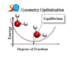
Steepest Descent (Gradient Descent)
This is the most simple technique to get the local minima or maxima of a function (in our case energy). One, simply, calculates the gradient (which is the direction of the steepest increase) and move in the negative direction of the gradient (which is simply the force in our case) to get to the minima which is what we desire. Then the value of the function (energy) is calculated at the new position and checked if it meets the convergence requirement or not, i.e. is the gradient 0 or not.
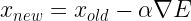
The coordinates our updated according to the equation:
where 


Conjugate Gradient
Do line minimizations in a direction which is a combination of the current gradient and the previous one
The coordinates our updated according to the equation:
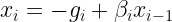
where

The different conjugate-gradient methods provide different ways to choose
; they involve dot products of current and previous gradients, e.g., Polak-Ribiere:


Now as you must have noticed by now, you would need the gradient of energy, i.e. the forces, to make the above algorithms work for geometry optimization using QE. Now QE can calculate and give you the forces as well as the total energy, so we have a way to access all the necessary information we are going to need.
A few questions that can come to mind regarding the above algorithms are answered below:
Using the gradient vector or the gradient unit vector?
Now in most of the literature, people generally use gradient vector but I also found some literature using gradient unit vectors for the descent direction. So I ran some calculations using that but the results didn’t offer anything conclusive. It didn’t seem to make any much of a difference. The code and results are shown below. I guess I would stick with using the gradient vector rather than unit vectors.
Constant step-length or adaptive step-length
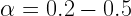
Now ideally the step-length
However, even in inexact line search you would have to calculate the total energy and gradients and this leads to a increased computation time. In a popular method known as backtracking line search you start with a large
But in my experience, if you start out with a good approximation to the starting geometry then the advantage provided by the starting large step-length is nullified by the need of making it smaller once you’re near the minimum. That is after taking the first large step, let’s say you’re now in the vicinity of the minimum. Now if you take the same large step-length then you would overshoot the minimum and energy will increase. So you would iteratively make
If you decide to run some calculations with constant step-length, here’s what I would suggest on how to choose it. First run a simple total energy calculation on your initial system and calculate the forces. This would give you an idea of how good is your starting approximation. If the forces are very low then this means you are close to the final (optimized) geometry. Based on this information you can decide on how big a step-length you’d need. For example, for the case of H2 molecule I found that using constant 

So these were the merits and demerits of both the constant or adaptive step length.
Parallelization:
Another idea that I have, is to parallelize the process of choosing the 
Comparing the results with the BFGS algorithm as implemented in Quantum ESPRESSO
Unfortunately, none of the Conjugate gradient or Steepest Descent variations mentioned here could come even close to BFGS algorithm as implemented in Quantum ESPRESSO. For small systems such as H2, N2 or O2, the results were comparable. But for systems with more degrees of freedom such as ZnS, CdS, Zn3S3, the convergence towards the minima took ages as compared to BFGS. The results are given below. I mean of course I expected it (CG and SD) to be slow but not this slow. So this was rather frustrating as I spent like a week working on this: writing codes for different variations, troubleshooting and running test calculations. I understand that there could be some problems with my implementations of Conjugate Gradient and Steepest Descent too. But this seems rather unlikely. However, if you’re reading this and have some suggestions or find some faults, please do let me know. Anyway my next goal is to implement the BFGS algorithm and see how does that fare in comparison to the one implemented by QE. QE uses trust region based BFGS, while I’m planning on first implementing it with an inexact line search using the wolfe conditions and bracketing and zooming the suitable
Using Wolfe conditions or not?
So as I mentioned before the suitable step-length should satisfy some set of conditions. However, I read that if you are using backtracking line search as the method for inexact line search for suitable
So I’ve spent quite some time discussing the various aspects of implementing a geometry optimization scheme using QE or any other DFT package. There are still lot’s of stuff that I didn’t cover, like using the cartesian coordinates or internal coordinates, etc. Anyway, the following are the various codes (shell scripts if you will) that I used for implementing various schemes. The scripts should be easily runnable on any Linux. You would have to just set the correct pw.x path and pseudopotential path. I’ve tried to provide useful comments in the code. Hope that helps.
Steepest Descent (with inexact line search for 1d optimization of step length)
The following is a shell script to implement Steepest Descent using backtracking line-search. In this code the value of
run.sh:
#!/bin/bash
#Script to find the optimized coordinates of a molecule/cluster using the Steepest Descent (Gradient Descent) algorithm interfaced with Quantum ESPRESSO
tol=$1
a=1
echo "A" > a.txt
chmod u+x scfCreator.sh
#--------------------------------
#Algorithm
#---------------------------------
#1. Run an SCF calculation using the user given starting geometry (atomic coordinates and PP info, etc.)
#2. Extract the information of forces acting on each of the atoms as that would give us the gradient of energy for each atom.
#3. Update the atomic coordinates for the nth atom using:
#   x{i,n}_new=x{i,n}_old + aF{i,n}
#  where i is for the ith coordinate and n is for nth atom and F is the force, i.e. negative of gradient, a is somescaling factor
#4. Keep repeating until the forces are minimized

#Find out no. of atoms
nat=$(awk '{for (I=1;I<=NF;I++) if ($I == "nat") {print $(I+2)};}' geom.in)
#Create an SCF file with the initial coordinates


iter=1
grep -A $nat 'ATOMIC_P' geom.in >coordIter$iter.txt
flag=1
while [ $flag == 1 ]
do
flag=0


iter1=$(($iter+1))
./scfCreator.sh 55 6 6 6 38 Iter$iter coordIter$iter.txt
mpirun '/mnt/oss/dmishra_du/QE/qe-6.1/bin/pw.x' -inp scfIter$iter.in> scfIter$iter.out
echo "Forces" >forcesIter$iter.txt
#echo "ATOMIC_POSITIONS {angstrom}" >coordIter$iter1.txt

if [ $iter != 1 ]
then
        E1=$(awk '{for (I=1;I<=NF;I++) if ($I == "!") {print $(I+4)};}' scfIter$iter.out)
        E0=$(awk '{for (I=1;I<=NF;I++) if ($I == "!") {print $(I+4)};}' scfIter$(($iter-1)).out)
if (( $(bc <<< "$E1 > $E0") ))
then
        a=$( echo "$a/2"|bc -l)
        iter=$(($iter-1))
else
        a=1
fi
#a=$( echo "$a/(($Fn1-($Fn01))*($Fn1-($Fn01))+($Fn2-($Fn02))*($Fn2-($Fn02))+($Fn3-($Fn03))*($Fn3-($Fn03)))"|bc -l)
fi
echo "ATOMIC_POSITIONS {angstrom}" >coordIter$(($iter+1)).txt

#Run a loop for no. of atoms
for (( n=1; n<=$nat; n++ ))
do

        species=$(grep -A $nat 'ATOMIC_PO' coordIter$iter.txt | sed '1d' | awk "NR==$n{print}" |awk  '{print $1}' )
        #Atomic positions at the start of this iteration
        x1=$(grep -A $nat 'ATOMIC_PO' coordIter$iter.txt | sed '1d' | awk "NR==$n{print}" |awk  '{print $2}' )
        x2=$(grep -A $nat 'ATOMIC_PO' coordIter$iter.txt | sed '1d' | awk "NR==$n{print}" |awk  '{print $3}' )
        x3=$(grep -A $nat 'ATOMIC_PO' coordIter$iter.txt | sed '1d' | awk "NR==$n{print}" |awk  '{print $4}' )
        #Extract the ith component of force of the nth atom
        Fn1=$(grep "atom    $n" scfIter$iter.out | awk '{for (I=1;I<=NF;I++) if ($I == "atom") {print $(I+6)};}')
        Fn2=$(grep "atom    $n" scfIter$iter.out | awk '{for (I=1;I<=NF;I++) if ($I == "atom") {print $(I+7)};}')
        Fn3=$(grep "atom    $n" scfIter$iter.out | awk '{for (I=1;I<=NF;I++) if ($I == "atom") {print $(I+8)};}')

        echo "$species      $Fn1   $Fn2   $Fn3" >>forcesIter$iter.txt

#If the force is less than the given threshold then don't update coordinate
#else update the coordinates using the formula in step 3. and alert the flag

        if (( $(bc <<< "${Fn1#-} >= $tol") ))
        then
                x1=$( echo "$x1+$a*$Fn1"|bc)
                flag=1

        fi
        if (( $(bc <<< "${Fn2#-} >= $tol") ))
        then
                x2=$( echo "$x2+$a*$Fn2"|bc)
                flag=1
        fi
        if (( $(bc <<< "${Fn3#-} >= $tol") ))
        then
                x3=$( echo "$x3+$a*$Fn3"|bc)
                flag=1
        fi

        echo $a >> a.txt
        if [ $n == $nat ]
        then
                echo "__________________" >>a.txt
        fi

        echo "$species      $x1   $x2   $x3" >>coordIter$(($iter+1)).txt
done
#If flag is not raised the geometry is optimized geometry else go bac to SCF calculation with updated coordinates
iter=$(($iter+1))
echo $flag >>flag.txt
done
Conjugate Gradient (with adaptive step length)
The following shell script implements the Conjugate Gradient algorithm using backtracking line search by interfacing with Quantum Espresso.
run.sh
#!/bin/bash
#Script to find the optimized coordinates of a molecule/cluster using the Conjugate Gradient algorithm interfaced with Quantum ESPRESSO
#Tolerance entered by the user
tol=$1
#Step-length \alpha
a=1
#Value of step-length at each iteration
echo "A" > a.txt
#Compile the input file creating script
chmod u+x scfCreator.sh
#--------------------------------
#Algorithm
#---------------------------------
#1. Run an SCF calculation using the user given starting geometry (atomic coordinates and PP info, etc.)
#2. Extract the information of forces acting on each of the atoms as that would give us the gradient of energy for each atom.
#3. Update the atomic coordinates for the nth atom using:
#   x{i,n}_new=x{i,n}_old + aF{i,n}
#  where i is for the ith coordinate and n is for nth atom and F is the force, i.e. negative of gradient, a is somescaling factor
#4. Keep repeating until the forces are minimized

#Find out no. of atoms
nat=$(awk '{for (I=1;I<=NF;I++) if ($I == "nat") {print $(I+2)};}' geom.in)
#Create an SCF file with the initial coordinates


iter=1
grep -A $nat 'ATOMIC_P' geom.in >coordIter$iter.txt
flag=1
while [ $flag == 1 ]
do
flag=0


iter1=$(($iter+1))
./scfCreator.sh 50 6 6 6 24 Iter$iter coordIter$iter.txt
'/home/manas/qe-6.1/bin/pw.x' <scfIter$iter.in> scfIter$iter.out
echo "Forces" >forcesIter$iter.txt


if [ $iter != 1 ]
then
	E1=$(awk '{for (I=1;I<=NF;I++) if ($I == "!") {print $(I+4)};}' scfIter$iter.out)
	E0=$(awk '{for (I=1;I<=NF;I++) if ($I == "!") {print $(I+4)};}' scfIter$(($iter-1)).out)
if (( $(bc <<< "$E1 > $E0") ))
then
	a=$( echo "$a/2"|bc -l)
	iter=$(($iter-1))
fi
#a=$( echo "$a/(($Fn1-($Fn01))*($Fn1-($Fn01))+($Fn2-($Fn02))*($Fn2-($Fn02))+($Fn3-($Fn03))*($Fn3-($Fn03)))"|bc -l)
fi

echo "ATOMIC_POSITIONS {angstrom}" >coordIter$(($iter+1)).txt
#Run a loop for no. of atoms
for (( n=1; n<=$nat; n++ ))
do

        species=$(grep -A $nat 'ATOMIC_PO' coordIter$iter.txt | sed '1d' | awk "NR==$n{print}" |awk  '{print $1}' )
	#Atomic positions at the start of this iteration
	x1=$(grep -A $nat 'ATOMIC_PO' coordIter$iter.txt | sed '1d' | awk "NR==$n{print}" |awk  '{print $2}' )
	x2=$(grep -A $nat 'ATOMIC_PO' coordIter$iter.txt | sed '1d' | awk "NR==$n{print}" |awk  '{print $3}' )
	x3=$(grep -A $nat 'ATOMIC_PO' coordIter$iter.txt | sed '1d' | awk "NR==$n{print}" |awk  '{print $4}' )
	#Extract the ith component of force of the nth atom
	Fn1=$(grep "atom    $n" scfIter$iter.out | awk '{for (I=1;I<=NF;I++) if ($I == "atom") {print $(I+6)};}')
	Fn2=$(grep "atom    $n" scfIter$iter.out | awk '{for (I=1;I<=NF;I++) if ($I == "atom") {print $(I+7)};}')
	Fn3=$(grep "atom    $n" scfIter$iter.out | awk '{for (I=1;I<=NF;I++) if ($I == "atom") {print $(I+8)};}')

	echo "$species      $Fn1   $Fn2   $Fn3" >>forcesIter$iter.txt

	if [ $iter == 1 ]
	then
		d1=$Fn1
		d2=$Fn2
		d3=$Fn3
	else
		Fn01=$(grep "atom    $n" scfIter$(($iter-1)).out | awk '{for (I=1;I<=NF;I++) if ($I == "atom") {print $(I+6)};}')
	Fn02=$(grep "atom    $n" scfIter$(($iter-1)).out | awk '{for (I=1;I<=NF;I++) if ($I == "atom") {print $(I+7)};}')
	Fn03=$(grep "atom    $n" scfIter$(($iter-1)).out | awk '{for (I=1;I<=NF;I++) if ($I == "atom") {print $(I+8)};}')
		B1=$(echo "$Fn1*($Fn1-($Fn01))+$Fn2*($Fn2-($Fn02))+$Fn3*($Fn3-($Fn03))"|bc)
                B1=$(echo "$B1/(($Fn01*$Fn01)+($Fn02*$Fn02)+($Fn03*$Fn03))"|bc -l)

                d1=$(echo "$Fn1+$B1*$d1"|bc)
                d2=$(echo "$Fn2+$B1*$d2"|bc)
                d3=$(echo "$Fn3+$B1*$d3"|bc)

	fi

#If the force is less than the given threshold then don't update coordinate
#else update the coordinates using the formula in step 3. and alert the flag

	if (( $(bc <<< "${Fn1#-} >= $tol") ))
	then
		x1=$( echo "$x1+$a*$d1"|bc)
		flag=1

	fi
	if (( $(bc <<< "${Fn2#-} >= $tol") ))
	then
		x2=$( echo "$x2+$a*$d2"|bc)
		flag=1
	fi
	if (( $(bc <<< "${Fn3#-} >= $tol") ))
	then
		x3=$( echo "$x3+$a*$d3"|bc)
		flag=1
	fi

	echo $a >> a.txt
	if [ $n == $nat ]
	then
		echo "__________________" >>a.txt
	fi

	echo "$species      $x1   $x2   $x3" >>coordIter$(($iter+1)).txt
done
#If flag is not raised the geometry is optimized geometry else go bac to SCF calculation with updated coordinates
iter=$(($iter+1))
echo $flag >>flag.txt
done
scfCreator.sh
The following script creates an scf input file for QE. It takes various info (Ecut, kx, ky, kz, nbnds and filename) as parameters. To make it work on your system just modify the pseudo_dir attribute giving the path to the pseudopotential files.
#!/bin/bash
#SCF input file creator for a given value of Ecut and kx,ky,kz, nbnd and filename

#Values of Ecut
pwcut=$1
pwrho=$(($pwcut*10))

#Values of k points
kx=$2
ky=$3
kz=$4

#no. of bands
nb=$5

#filename
suffix=$6
file=scf$suffix.in

coordFile=$7

echo '&CONTROL
    calculation = "scf"
    max_seconds =  8.64000e+08
    pseudo_dir  = "/home/manas/Scripts/GGA_SemiConductor/pseudopot"
    outdir      = "temp"
    tprnfor     = .TRUE.
    tstress     = .TRUE.

/' >$file

echo '&SYSTEM' >>$file
#Find out the lattice information from the geom.in file and append that to input file (Using sed non-inclusive)
sed -n '/&SYSTEM/,/\//p' geom.in | sed '1d;$d' >> $file


echo '
    degauss     =  1.00000e-02
    ecutrho     =  '$pwrho'
    ecutwfc     =  '$pwcut'
    occupations = "fixed"
    smearing    = "gaussian"
    nbnd        =  '$nb'
/' >>$file
echo '
&ELECTRONS
    conv_thr         =  1.00000e-06
    electron_maxstep = 200
    mixing_beta      =  7.00000e-01
    startingpot      = "atomic"
    startingwfc      = "atomic+random"
/

K_POINTS {gamma}
 '$kx'  '$ky'  '$kz'  0 0 0
'>> $file

echo 'ATOMIC_SPECIES' >>$file

sed -n '/ATOMIC_S/,/ATOMIC_P/p' geom.in | sed '1d;$d' >> $file

sed -n '/ATOMIC_P/,//p' $coordFile  >> $file
References:
http://www.quantum-espresso.org/
https://en.wikipedia.org/wiki/Line_search
https://en.wikipedia.org/wiki/Gradient_descent
https://en.wikipedia.org/wiki/Conjugate_gradient_method
https://en.wikipedia.org/wiki/Wolfe_conditions
https://en.wikipedia.org/wiki/Backtracking_line_search
https://en.wikipedia.org/wiki/Quasi-Newton_method
https://en.wikipedia.org/wiki/Broyden–Fletcher–Goldfarb–Shanno_algorithm
I’m a physicist specializing in computational material science with a PhD in Physics from Friedrich-Schiller University Jena, Germany. I write efficient codes for simulating light-matter interactions at atomic scales. I like to develop Physics, DFT, and Machine Learning related apps and software from time to time. Can code in most of the popular languages. I like to share my knowledge in Physics and applications using this Blog and a YouTube channel.