I have written a code that will calculate the coefficients of the polynomial that will best fit a given set of data-points.

The procedure is based on least square approximation, which, in simple words,works by finding a polynomial that is at a minimum distance possible from all the points.

Let’s say you have the x-axis points stored in a matrix, ‘x’ & the y-axis points stored in a matrix ‘y’ and you want to find a polnomial of n-th degree that best fits the data. Then the following code returns the values of the coefficients of the best fit-polynomial.

CODE:

//Polynomial Fitting
//To fit a given set of data points to an n-degree polynomial
//Written By: Manas Sharma (www.bragitoff.com)
funcprot(0);
function A=npolyfit(x,y,n)
    format(6);
    N=size(x);
    if N(2)>N(1) then
        N=N(2)
    else
        N=N(1);
    end
    X(1)=N;
    for i=1:2*n
        X(i+1)=0;
        for j=1:N
            X(i+1)=X(i+1)+x(j)^i;
        end 
    end
    for i=1:n+1
        for j=1:n+1
            B(i,j)=X(i+j-1)
        end
    end
    disp(B);
    for i=0:n
        C(i+1)=0;
        for j=1:N
            C(i+1)=C(i+1)+(x(j)^i)*y(j);
        end
    end
    C=-C;
    disp(C);
    A=linsolve(B,C);
endfunction
    

Sample Demo:

x=[1,2,3,4,5];
y=[1,8,27,64,125];
a=npolyfit(x,y,3)

In the above code I have a set of data-points for the x-axis being stored in the matrix ‘x’, and the y-axis points in the matrix ‘y’. As you can clearly see that the equation of y should be x^3 as it is just the cube of the x-axis points, so I have given the third argument n=3 when I called the function npolyfit.

Output:

a  =

0.000
– 0.000
0.000
1.

The output is a matrix whose fourth element is 1 while the first three are 0. Since the (n+1)th element of the matrix corresponds to the coefficient of x^n(where n goes from 0 to n), therefore we get the coefficient of x^3 to be 1.

Hence, we know that the polynomial which best fits the data is x^3+0*x^2+0*x^1+0*x^0.

The last example was a little bit straight-forward. Now let’s try something a little more tricky.

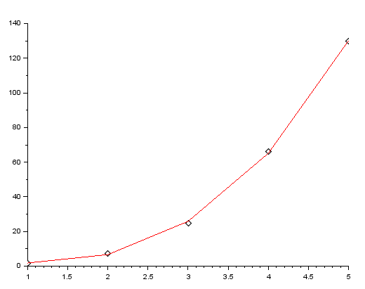
x=[1,2,3,4,5];
y=[1.6,7.5,24.6,66,130];
a=npolyfit(x,y,3)

Now this time we can’t exactly calculate the polynomial ourselves, but by intuition we can tell that the best fit would be a polynomial of 3rd degree. Why? Because if you compare the data-points with the previous example then you can see that they are only just a little bit off.

Output:

a  =

5.64
– 6.264
1.486
0.95
In case you are wondering if it’s correct or not or maybe you want to plot it then you can define a function f(x) which is a polynomial of degree 3 with the above coefficients:

deff('g=f(x)','g=0.95*(x^3)+1.486*(x^2)-6.264*(x)+5.64')

Then create a matrix ‘yfit’ which stores the fitted points:

yfit=f(x);

And then plot the original/observed data-points as markers/dots:

plot2d(x,y,-5)

and then plot the fitted data points as red line:

plot2d(x,yfit,5)

Output:

I have created a module in SCILAB which contains the above macro, and once installed can be used as an in-built function. You can download it from here: https://atoms.scilab.org/toolboxes/curvefit

Leave your questions/suggestion/corrections in the comments section down below and I’ll get back to you soon.